Building a Plotly Dashboard on a Lakehouse using Apache Iceberg & Arrow
In my last blog, I highlighted the advantages of using low-code platforms like Streamlit to build full-stack data applications on a data lakehouse. This tutorial focuses on building a Python-based dashboard using a similar low-code framework called Plotly Dash. Dash open source allows us to develop interactive data apps using pure Python, thereby taking off the dependency on JavaScript, which was typically used in the past to build full-stack visualization solutions.
A couple of ways to build a Dash app are by consuming data from sources such as CSV files, databases, API/web services, etc. However, this blog will attempt to build a dashboard using data directly from a data lakehouse. If you hear about a lakehouse for the first time, here is a blog to navigate the basics.
At a high level, a lakehouse is a type of architectural pattern that brings in data management capabilities of warehouses and scalability & low-cost factors of data lakes using open table formats for storage like Apache Iceberg. A lakehouse architecture provides flexibility in choosing the right set of technical components (tools) for the right use case.

Before we delve into the practical aspects of this application, let’s theoretically understand the three (3) main components that will be needed to build the dashboard. Again, we can use any other options for these components in a lakehouse.
1. Storage (Data Source)
With an open table format such as Apache Iceberg, we have the flexibility to treat data as a separate, independent tier and can bring any compute (that supports Iceberg) to cater to a range of analytical use cases such as BI reports and machine learning. It also enables our data architecture to be future-proof. How, you may ask?

So, let’s say, today, you are using Iceberg with an SQL engine for batch workloads, but in the future, you want to deal with real-time data and need to use a stream processing engine like Apache Flink. With a traditional data architecture, this might involve exporting the data from a warehouse to a data lake or having to deal with other things in your current architecture. With data in open formats, you only have to point the compute engine to the data and not vice versa.
2. Compute Engine
The next important component in our architecture is the compute engine. It is non-trivial to understand that Iceberg is a table format specification (a set of APIs) on top of storage systems like data lakes. So, the responsibility to process and transform data lies in the hands of a compute engine. Unlike a data warehouse where only the warehouse’s compute engine can access and process data efficiently, in a lakehouse, data is stored in open table & file formats like Iceberg and Parquet. So, depending on the analytical use case, we can use the right compute.

We will use Dremio Sonar — a data lake SQL engine optimized for business intelligence and ad hoc/exploratory workloads for this demo. Another important reason for choosing Dremio Sonar as the compute is its support for Apache Arrow Flight SQL protocol (more on it in the next section), which enables faster columnar data access & retrieval.
3. Arrow Flight/Flight SQL
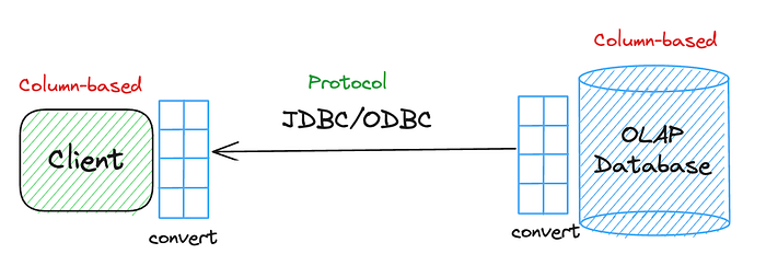
Arrow Flight is a client-server framework to simplify high-performance transport of large datasets over network interfaces. ODBC/JDBC has been the de facto protocol to transfer data across systems. However, the problem with these two protocols is that they are particularly designed to deal with row-based data. However, today, with OLAP analytics, specifically with huge data volumes, the storage choice is columnar. Additionally, most of the client tools involved with OLAP databases also want to leverage the same columnar benefits for performance gains, but the problem is there is no ‘standard’ for columnar data transport.
Here’s a common scenario where we lay out the problem.

Let’s say we store data in a column-based OLAP DB and use a columnar client to consume data from it. The goal is to send this columnar data over the ODBC/JDBC protocol to the client. To do so, we will need to convert the columnar data into rows first, and then, on the client side, we will need to convert it back to columns again. This entire process of serialization/deserialization can take anywhere from 60–90% of the transfer time, significantly impacting the performance.
This is where the Arrow Flight framework comes into play and acts as a standard for columnar data transport.
Ok, so, what is Arrow Flight SQL then?
Arrow Flight SQL is the protocol for interacting with SQL databases built on Arrow Flight. In simpler terms, Arrow Flight SQL allows databases to use the Flight protocol and standardizes various database-related activities, such as — how to do query execution, how to submit a query and get results back, etc. By providing a defined way to do various types of operations with databases, Arrow Flight SQL eliminates the need for each client to interpret things in their own way, thereby establishing a standard for client database access. If you are interested in learning more about Arrow & its sub projects, I did a walkthrough of it at Subsurface: The Data Lakehouse conference.
Now that we have all three components for our mini project let us see how to build this lakehouse architecture.
Lakehouse Architecture

Here’s how we will approach our problem — building the Plotly dashboard using data directly from a lakehouse.
- The data files are stored in an S3 data lake as Parquet files.
- We create an Iceberg table using Dremio Sonar as the compute engine.
- Dremio Sonar enables support for Arrow Flight SQL endpoints. Using this endpoint, we can query Iceberg data and consume it as Arrow batches.
- Finally, we will use this data to build our Plotly application.
Create Iceberg Table
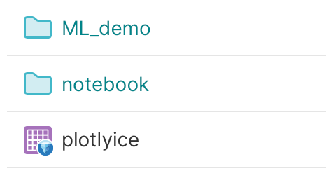
The screenshot below presents a lineage of the data files. As we can see, the files are currently stored in a S3 data lake as a folder.

We can use any compatible compute engine to create our first Iceberg table. In this case, we use Dremio Sonar, which provides an easy interface to connect to the data lake to create Iceberg tables. However, we can use any other compute, such as Spark, Trino, or Presto.
We will use the CTAS command in Dremio Sonar to create the Iceberg table.

By default, Sonar will create this table in Dremio’s Arctic catalog. Note that a catalog is a pre-requisite to create an Iceberg table & it brings atomicity and consistency guarantees with every transaction. Again, we can choose compatible catalogs like AWS Glue or Hive metastore here.
If we check the catalog, we can see all the existing Iceberg tables and the newly created table called ‘plotlyice’.

Install the required Libraries
Let’s install and import all the necessary libraries required for us to build the dashboard. Specifically, we need the following:
- PyArrow
- Arrow Flight
- Plotly Express
- Dash
pip install pyarrow
pip install plotly
import os, pandas as pd
from pyarrow import flight
import pyarrow as pa
from os import environ
import plotly.express as px
import plotly.graph_objects as go
import dash
import dash_core_components as dcc
import dash_html_components as html
import dash_bootstrap_components as dbc
from dash import dash_table
from dash.dependencies import Input, Output, StateFlight SQL API Call
Now, let’s make the API call to Dremio’s Flight SQL endpoint and consume the data from the Iceberg table as an Arrow table.
token = environ.get('token', 'Dremio_Token')

headers = [
    (b"authorization", f"bearer {token}".encode("utf-8"))
    ]

client = flight.FlightClient('grpc+tls://data.dremio.cloud:443')
options = flight.FlightCallOptions(headers=headers)

sql ='''SELECT * FROM arctic.plotlyice LIMIT 200000'''

info = client.get_flight_info(flight.FlightDescriptor.for_command(sql + '-- arrow flight'),options)

reader = client.do_get(info.endpoints[0].ticket, options)

batches = []
while True:
    try:

        batch, metadata = reader.read_chunk()
        batches.append(batch)
    except StopIteration:
        break
data = pa.Table.from_batches(batches)
If you are interested in understanding how clients interacts with Dremio’s Arrow Flight SQL endpoint, here is a resource.
Once we get the data as an Arrow table, we then convert it into a Pandas dataframe object so we can use it directly in our visualization objects.
The ability to use Arrow tables directly in a Plotly/Dash object can help reduce this additional conversion and data copy. At the time of writing this blog, there are initial discussions around this support via Python’s new data interchange protocol.
Create Visualizations
Finally, we can use the data to create the visualization objects for our dashboard. Here’s a snippet.
html.Div(
            children=[
                dcc.Graph(
                    figure=px.bar(avg_fare_by_passenger_count, x='passenger_count', y='fare_amount', title='Average Fare Amount by Passenger Count')
                     .update_traces(marker_color=colors['chart'])
                .update_layout(template=template, font=dict(family="DM Sans", size=12, color="#1F2937")),
                    config={"displayModeBar": False},
                ),
                dcc.Graph(
                    figure=px.scatter(df, x='trip_distance_mi', y='total_amount', title='Trip Distance vs Total Amount' )
                    .update_traces(marker_color=colors['chart'])
                    .update_layout(template=template, font=dict(family="DM Sans", size=12, color="#1F2937")),
                    config={"displayModeBar": False},
                ),
            ],
            style={"display": "flex", "justify-content": "space-between", "margin-bottom": "30px"}
)
Query Interface
As part of this dashboard, we also wanted to provide a query interface so users can do some level of ad hoc analysis on the Iceberg tables directly. All these queries use Dremio Sonar as the compute engine to interact with the Iceberg table.
# Using a Textfield for input query & Table component for rendering output in Plotly
html.Div(
            children=[
         dcc.Textarea(
            id='input-query',
            placeholder='Enter SQL query...',
            style={'width': '100%', 'height': '100px', 'margin-bottom': '10px'}
        ),

        html.Button('Run Query', id='run-query-button', n_clicks=0),

        dash_table.DataTable(
            id='data-table',
            style_table={'overflowX': 'auto'},
            style_cell={'textAlign': 'left'},
        )
            ],

        ),

# Logic to get the data from the Iceberg table based on the input query

        while True:
            try:
                batch, metadata = reader.read_chunk()
                batches.append(batch)
            except StopIteration:
                break
        data = pa.Table.from_batches(batches)
        df = data.to_pandas()
        data_new = df.to_dict('records')
        columns = [{'name': col, 'id': col} for col in df.columns]

        return data_new, columns

    default_data = []
    default_columns = [{'name': 'No Data', 'id': 'nodata'}]
    return default_data, default_columns
Dashboard
Here’s our final dashboard with all the 4 visualization objects.

By building the dashboard directly on the data lakehouse, we achieve certain advantages:
- Reduced data wait requests: By having direct access to the data, we do not have to wait for data pipelines to deliver new or changed data. This improves the time-to-insight process and makes analysis relevant.
- No unmanageable data copies: With the traditional way of building reports, data is usually moved across various systems before it is made available to analysts, leading to many data copies. With a lakehouse, this aspect is controlled.
- Better Cost: Since data is stored in cloud object stores such as S3, we can scale storage as we like. On top of monetary costs, the costs of maintaining ETL pipelines, creating extracts, etc., are eliminated.
If you want to use the code and try building something similar for your use cases, here is the GitHub repository.
